New developments on instability analysis for large chaotic systems
What are the Lyapunov vectors?
Chaos is often characterized by Lyapunov exponents, which quantify the rate of exponential growth of infinitesimal perturbations applied to trajectories. In general, $N$-dimensional systems have $N$ Lyapunov exponents $\lambda^{(1)} \geq \lambda^{(2)} \geq \cdots \geq \lambda^{(N)}$ depending on the direction of perturbations (Oseledec's theorem) [A,B]. The proper direction of perturbation for the exponent $\lambda^{(j)}$ is then called the Lyapunov vector $\pmb{v}^{(j)}$. The Lyapunov exponents are known to be related to various quantities and properties of chaos, such as the attractor dimension, the metric entropy, and the extensivity, and are much studied thanks to the established algorithm to compute Lyapunov exponents [C]. In contrast, much less is known for the Lyapunov vectors, for which no such practical algorithm had existed for a long time, until Ginelli and coworkers invented in 2007 an efficient algorithm that can also be used for large chaotic systems [D]. (In passing, since the true Lyapunov vectors had long remained unavailable, the Gram-Schmidt orthonormal basis, which is obtained as a by-product of the standard algorithm to compute Lyapunov exponents, has sometimes been called Lyapunov vectors in the literature. We however stress that the Gram-Schmidt vectors are different from the Lyapunov vectors even qualitatively, so one should always use the true Lyapunov vectors. To distinguish, the true Lyapunov vectors are sometimes called the covariant Lyapunov vectors.)
The relationship between Lyapunov exponents and vectors is analogous to that between eigenvalues and eigenvectors, so the Lyapunov vectors may potentially carry as important information as the Lyapunov exponents. Indeed, one can obtain the following information from the Lyapunov vectors $\pmb{v}^{(j)}$, for example: "spatial structure of each Lyapunov mode (instability mode)" and "degree of hyperbolicity of a given dynamical system and/or a Lyapunov mode". The former is encoded in $\pmb{v}^{(j)}$'s vector components, while for the latter one can measure the angle spanned by a pair of Lyapunov vectors. Thus analyzing Lyapunov vectors besides the Lyapunov exponents, which we call the Lyapunov vector analysis, can be a powerful tool to characterize various statistical aspects of large chaotic systems.
Discovery of collective Lyapunov modes
Large chaotic systems often exhibit non-trivial collective behavior, in which a collection of chaotically evolving elements shows a variety of time-dependent behavior at the macroscopic level [E]. Studying such systems by the Lyapunov vector analysis, we found a few "collective Lyapunov modes" that act collectively on the trajectory, amid the remaining $\mathcal{O}(N)$ "microscopic modes" which perturb only a few degrees of freedom without a macroscopic effect [1] (Movie 1). The collective and microscopic modes can be clearly defined and distinguished in terms of delocalization properties of the associated Lyapunov vectors. Since the collective modes are expected to characterize collective dynamics of the system, we believe they are useful to address fundamental questions regarding the effective dimension and the bifurcation structure of collective dynamics, as well as for applications such as control of chaos at the collective level.
Effective dimensions of dissipative systems
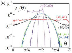
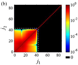
As another example of applications of the Lyapunov vector analysis, we numerically showed that the hyperbolicity of Lyapunov modes determines an effective number of degrees of freedom for dissipative systems, including dissipative partial differential equations (PDEs) [2]. In dynamical systems theory, though PDEs are formally infinite-dimensional, it is argued that trajectories in such systems are first exponentially attracted to a finite-dimensional invariant manifold called the inertial manifold, so the time evolution thereafter can be in principle described by a finite number of degrees of freedom [F]. The existence of such a finite-dimensional inertial manifold has indeed been proved mathematically for some PDEs like the Kuramoto-Sivashinsky (KS) equation, but such proofs do not tell us the dimensionality or the structure of the inertial manifold. On the other hand, we intuitively expect that such perturbations that kick trajectories out of the inertial manifold will decay without any influence on the dynamics inside the manifold. This suggests a splitting of tangent space into the Lyapunov vectors living inside the inertial manifold and the others. This has indeed been shown the case: measuring the angle between Lyapunov vectors for prototypical dissipative systems like the KS equation, we found that the tangent space consists of "physical Lyapunov modes" that have tangencies with other physical modes occasionally, and the remaining "spurious Lyapunov modes", associated with negative Lyapunov exponents and characterized by the absence of tangencies with any physical mode [2] (Fig. 1). The manifold constituted by the physical modes can be interpreted as a local approximation of the inertial manifold, which then indicates that the number of the physical modes is exactly the inertial manifold dimension. A similar separation between the physical and spurious modes can also be identified by analysis of a collection of unstable periodic orbits, being consistent with the conception that unstable periodic orbits constitute the skeleton of chaos [G]. Though a mathematical proof for this relation to the inertial manifold is certainly called for, our method seems to capture the inertial manifold for the first time numerically, which we expect is useful for both fundamental and practical purposes.
While the Lyapunov vector analysis is able to probe such interesting statistical properties of large chaotic systems, experimentally this remains totally inaccessible. We aim to overcome this difficulty and started to discuss possible approaches.
References
(Takeuchi Lab)
[1] K. A. Takeuchi, F. Ginelli, and H. Chaté, Phys. Rev. Lett. 103, 154103 (2009) [pdf, web]; K. A. Takeuchi and H. Chaté, J. Phys. A 46, 254007 (2013) [web, preprint].
[2] H.-l. Yang, K. A. Takeuchi, et al., Phys. Rev. Lett. 102, 074102 (2009) [pdf, web]; K. A. Takeuchi et al., Phys. Rev. E 84, 046214 (2011) [pdf, web].
[3] X. Ding, H. Chaté, P. Cvitanović, E. Siminos, and K. A. Takeuchi, Phys. Rev. Lett. 117, 024101 (2016) [pdf, web].
(other groups)
[A] J.-P. Eckmann and D. Ruelle, Rev. Mod. Phys. 57, 617 (1985) [web].
[B] E. Ott, Chaos in Dynamical Systems (Cambridge Univ. Press, Cambridge, 1993).
[C] I. Shimada and T. Nagashima, Prog. Theor. Phys. 61, 1605 (1979) [web]; G. Benettin et al., Meccanica 15, 9 (1980) [web].
[D] F. Ginelli et al., Phys. Rev. Lett. 99, 130601 (2007) [web]; F. Ginelli et al., J. Phys. A 46, 254005 (2013) [web].
[E] H. Chaté and P. Manneville, Prog. Theor. Phys. 87, 1 (1992) [web].
[F] P. Constantin et al., Integral Manifolds and Inertial Manifolds for Dissipative Partial Differential Equations (Springer, Berlin, 1988).
[G] P. Cvitanović et al., Chaos: Classical and Quantum (Niels Bohr
Institute, Copenhagen, 2016) [web].
Main contributors
K. A. Takeuchi